How to use XLOOKUP: Guide and Examples

If you’ve been using Excel for a while, you’ll undoubtedly have used one of its most useful functions – VLOOKUP.  This lookup function is invaluable when manipulating data or preparing reports in Excel.  If you’re already familiar with VLOOKUP, then you’ll love the new XLOOKUP function that Microsoft released in late 2019.  It overcomes some of the limitations of VLOOKUP and is easier to use.

Introduction

If you’ve never used VLOOKUP before, then get ready to learn about an extremely powerful function.  Once you’ve learned how the XLOOKUP function works and what it can be used for, you’ll wonder how you ever managed your spreadsheeting without it.

Note : XLOOKUP is only available in Excel for Microsoft 365. 
It is not available for Excel 2019 or prior versions.

What is the XLOOKUP function?

Before we look at the XLOOKUP function itself, let’s just first clarify what the term ‘lookup’ in general means when referring to spreadsheets and databases.  A ‘lookup table’ is normally a table that acts as a “master list” for something and you use it to look up a business value (like “Product Name”) using an identifier (like the “Product ID” column).  So, a ‘lookup function’ is simply a way of performing this lookup.  A typical example is an extract for a sales report which lists product_id and sales for a period.  On their own these two columns aren’t very useful, but if we can add product name, product category, sales rep, and other things, it is more useful for reporting purposes.  XLOOKUP can easily add all that extra information.

In its simplest form, the XLOOKUP function looks like this:

XLOOKUP(lookup_value,lookup_array,return_array)

where

• lookup_value: What you are looking for
• lookup_array: Where to find it
• return_array: What to return

The official Microsoft article on the XLOOKUP function is here.

XLOOKUP: Basic Exact Match

The easiest way to see how XLOOKUP works is to look at a simple example.  Here we have a table that shows Area Codes and the corresponding State/Territory.  The following formula looks up a value (in this case “Ohio”) and returns the correct Area Code:

=XLOOKUP(D3,B2:B313,A2:A313)

 

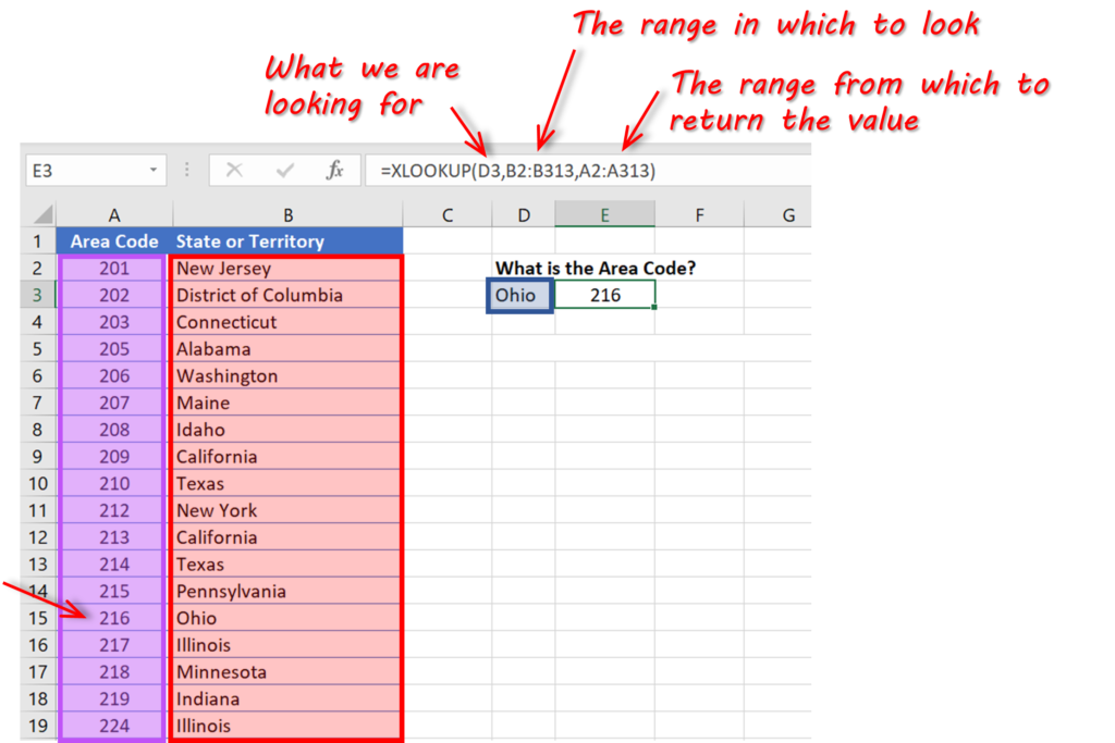
People familiar with VLOOKUP will immediately notice two things with this formula:

• To perform a basic exact match like this, only 3 arguments are needed. VLOOKUP needed an extra one to specify whether to use an approximate match (the default behavior) or an exact match.
• XLOOKUP can look up values to the left of the lookup array. This overcomes a big limitation with VLOOKUP, as users often had to re-arrange their columns to get the lookup array on the left.

XLOOKUP: Advanced variations

The basic exact match shown in the example above meets most users’ needs.  However, XLOOKUP includes some very useful options to cater for more complex situations.  The additional arguments are ‘if_not_found’, ‘match_mode’ and ‘search_mode’:

=XLOOKUP(lookup_value,lookup_array,return_array,[if_not_found],[match_mode],[search_mode])

XLOOKUP: Approximate Match

One of the more common uses of the advanced variations is when you need to look up an approximate match.  For this, we’ll need to specify the ‘match_mode’.  In the example below, we want to populate the grades that students will get based on their marks.  We can do it by entering this equation in C2:

=XLOOKUP(B2,$F$3:$F$7,$G$3:$H$7,,1)

Note that we’ve added a value of 1 for the ‘match_mode’ argument, which will return the index of the next largest item if an exact match isn’t found.  The full list of options is:

• 0 (default) Exact match. Will return #N/A if no match.
• -1 Exact match or next smaller item.
• 1 Exact match or next larger item.
• 2 Wildcard match (*, ?, ~)

XLOOKUP – return multiple values

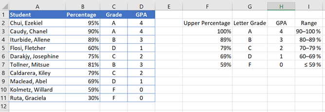
There is another thing to note about the equation.  We have specified the range that covers both the Letter Grade and GPA values for the return array.  This allows us to use a neat trick with XLOOKUP – returning multiple values with one formula.  When you press enter, you’ll see that the GPA value is automatically populated as well!

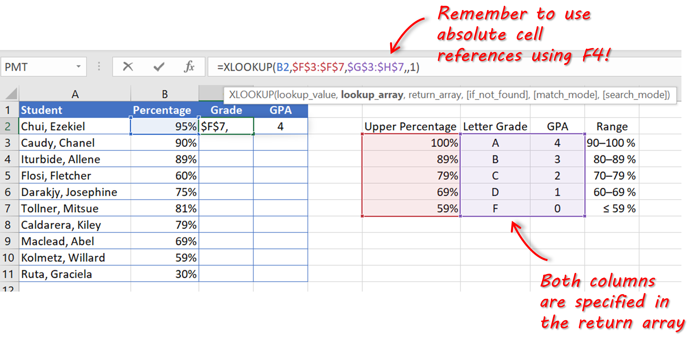
When we copy the formula into the other rows (remembering to specify absolute cell references), the Grades and GPA values are all correctly populated.

XLOOKUP: Not Found Message

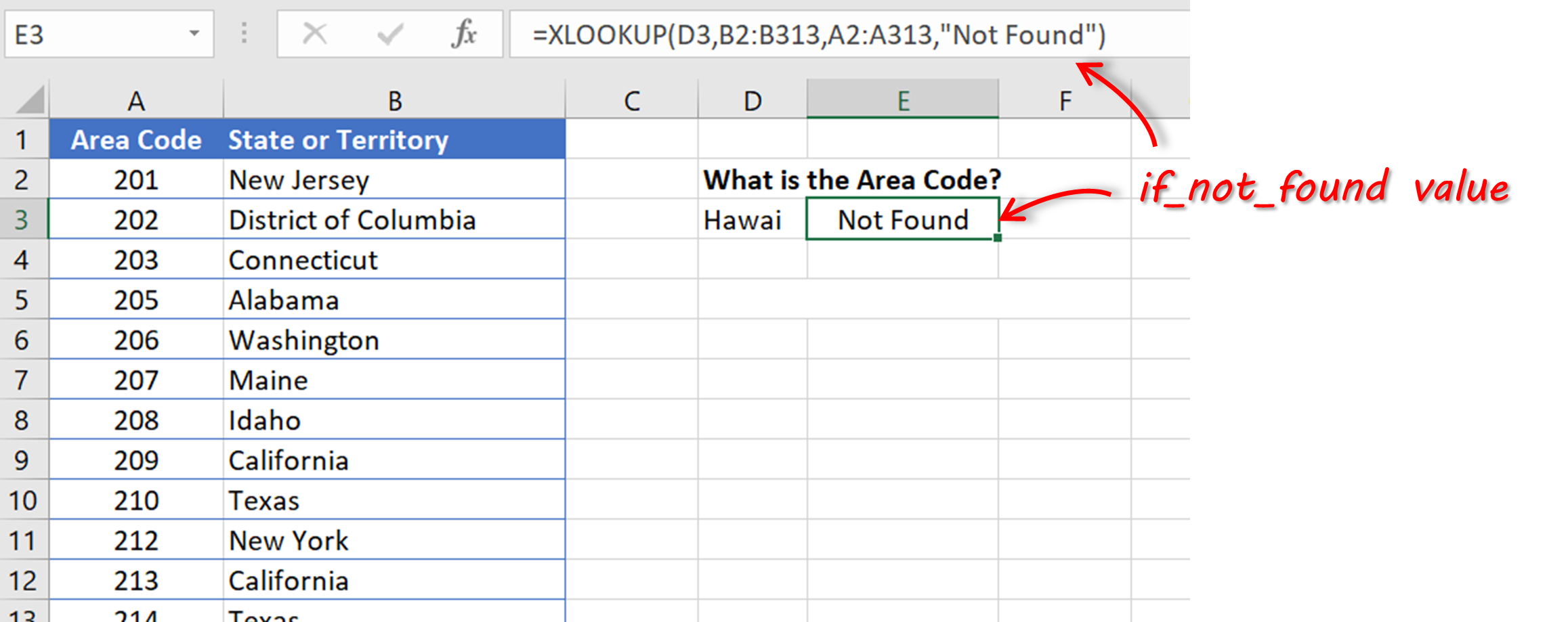
When the XLOOKUP function does not return a value, it displays the “#N/A” message in the cell.  This can be somewhat ambiguous for users – what does this mean? is this an error?  It’s therefore good practice to provide a more useful message.  Users familiar with the VLOOKUP function would often wrap the VLOOKUP statement inside an IFERROR function to return a friendly message.  HOWEVER, the XLOOKUP function makes it much easier to do this with the ‘if_not_found’ argument.

XLOOKUP(lookup_value,lookup_array,return_array,[if_not_found],[match_mode],[search_mode])

If we go back to our first exact match example and add a value for the ‘If_not_found’ argument, then a more useful message can be displayed to the end-user.

XLOOKUP: Search Mode

How do lookup functions handle the situation when the same value can appear more than once in the lookup array?  This situation is common in things like stock sheets when stock levels for products on a given day are appended to an existing list.

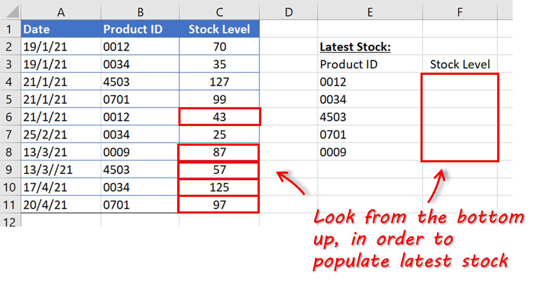
In the example below, we want to find the latest stock level for each product. The stock levels are updated periodically in the spreadsheet by adding new rows with the current date and stock level.  To get the latest stock level, we need to retrieve only the values from the most recent dates and ignore everything else.

The formula to do this is:

=XLOOKUP(E4,$B$2:$B$11,$C$2:$C$11,"Not Found",0,-1)

Note that we have set the ‘search_mode’ argument to a value of -1, which will perform the look-up from last to first. The default value is 1, which searches from first to last.

Putting it all together: a guided XLOOKUP example

In this simple example we’re going to start with some basic sales data and enhance it to calculate some useful business metrics:

• Commission per Sales Rep
• Sales per State

The sample data is here.  

The screenshot below shows our starting point – let’s assume that this was a sales extract from an accounting system for the previous month.

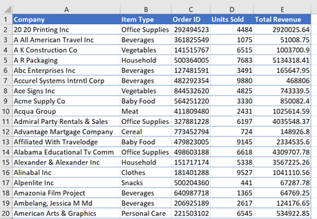
We want to add the following columns to the table:

• Company City
• Company State
• Sales Rep
• Commission Tier
• Commission Percentage
• Commission Amount

To add these extra columns, we need to use the following lookup tables:

• Company to Rep lookup
• Rep to Commission Tier lookup
• Product/Tier Commission lookup

In the example workbook, these are in a separate sheet called ‘lookups’

Step (1): add the City, State, Sales Rep columns

To add these columns, we can use the basic exact match form of XLOOKUP.  Remember that we can make use of one of XLOOKUP’s clever shortcuts and get all 3 columns by entering one formula in F2.  We do this by specifying the range $B$2:$D$501 in the company to sales rep lookup table.

=XLOOKUP(A2,lookups!$A$2:$A$501,lookups!$B$2:$D$501,"Not Found")

As soon as you enter the formula, it will ‘spill over’ into the next two columns, and return the relevant values.

Our formula includes absolute cell references, so we can copy these formulas all the way down for the rest of the rows:

Step (2) : add the Commission % column

In this example, the sales reps get paid a commission based on the type of product and the ‘commission tier’ that they are currently on.  So, for example, if Ezekiel Chui gets a customer order for household products, the commission he’ll earn will be 0.5% of the order value.

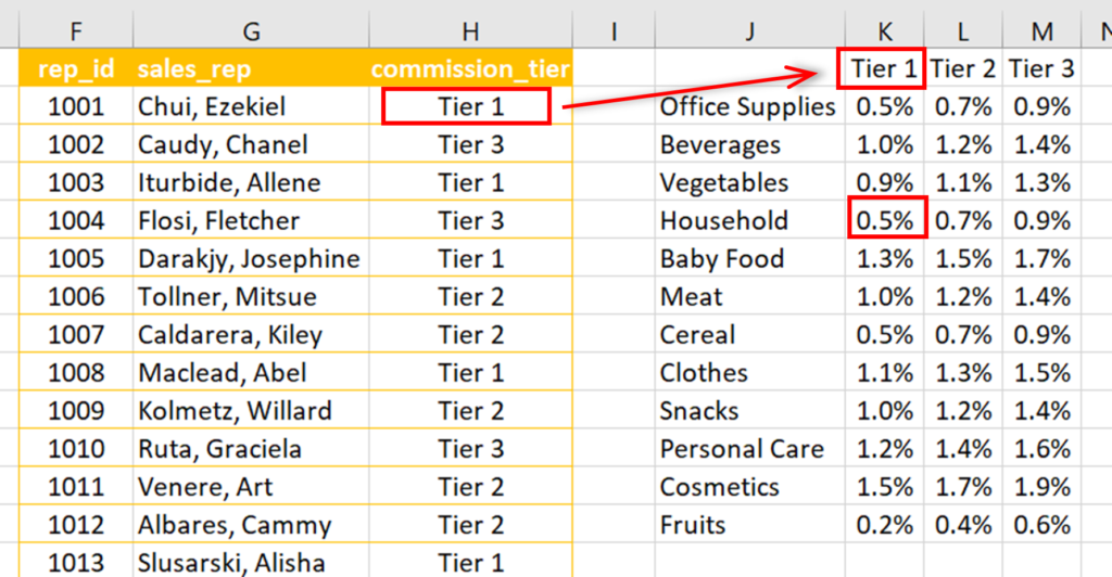
First, we’ll add a column to our table to retrieve the relevant sales rep commission tier for each order using a basic exact match lookup.  In cell I2 we can enter the following:

=XLOOKUP(H2,lookups!$G$2:$G$29,lookups!$H$2:$H$29,”Not Found”)

Now we can copy this cell for the other rows

Next, we need to get the commission percentage value for each order to work out the commission amount eventually.  To do this we’re going to perform a two-way lookup using a nested XLOOKUP function:

=XLOOKUP(I2,lookups!$K$1:$M$1,XLOOKUP('sales final'!B2,lookups!$J$2:$J$13,lookups!$K$2:$M$13))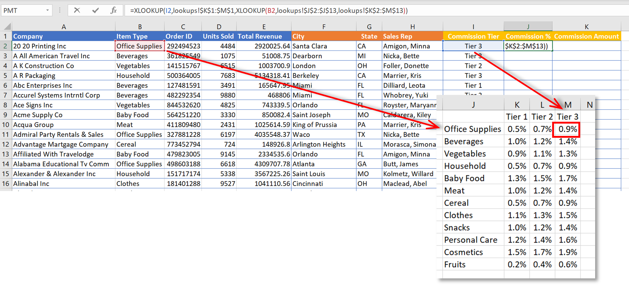

In the example, the “inner” XLOOKUP retrieves an entire row (all values for ‘Office Supplies’), which is handed off to the “outer” XLOOKUP as the return array.  The outer XLOOKUP finds the appropriate commission tier (Tier 3) and returns the corresponding value of 0.9%

We can now copy this formula to all the other rows to populate the ‘Commission %’ column:

NOTE: there is a way to populate the ‘Commission %’ column without using the ‘Commission Tier’ column by using an extra XLOOKUP nesting layer in the formula:

=XLOOKUP(XLOOKUP(H2,lookups!$G$2:$G$29,lookups!$H$2:$H$29),lookups!$K$1:$M$1,XLOOKUP(B2,lookups!$J$2:$J$13,lookups!$K$2:$M$13))

Step (3): calculate the Commission Amount

The final step is to simply calculate the amount of commission that each sales rep earns for each order:

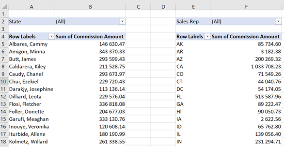
Step (4): summarise the data with pivot tables

Pivot tables are a great way to summarize this kind of data.  Here are a couple of examples:

Bonus tip: Dependent drop-down list using XLOOKUP

Here is another great way of using XLOOKUP – creating dependent drop-down lists.  We’re all familiar with using drop-down lists in applications.  As well as being a user-friendly way of adding or editing data, it’s also a very good way of maintaining data integrity. Only options from a ‘master’ lookup list can be chosen, and there is no risk of typos or other data entry errors.

This is a simple example that shows how to use XLOOKUP to create a drop-down list to select a country, and a second dependent drop-down list to choose a city.  So, if a user selects ‘USA’ from a drop-down list in the Country column, they should then select from a choice of New York, Dallas, or Miami in the City column.

Step (1): Create the Country drop-down

To create the Country drop-down, click on cell A3, and then click on the Data ribbon tab and then the Data Validation button.

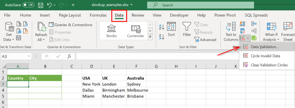
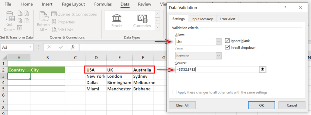
In the dialog box that is displayed, select “List” for the ‘Allow’ option, and in the ‘Source’, select the range where the countries are listed.  We can now copy this to the A4:A5 range.

Now when we click on a cell in the Country column, we can select from the drop-down list:

Step (2): Create the dependent City drop-down

To add the City drop-down, we’re going to use an XLOOKUP function.  To do this, select cell B3 and click on Data > Data Validation.  Once again, we select ‘List’, but this time in the ‘Source’ we’re going to enter the following formula, before clicking Ok.

=XLOOKUP(A3,$D$2:$F$2,$D$3:$F$5)

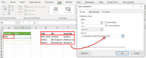
When you select B3 now, you’ll see that you can select from one of the three USA cities. 

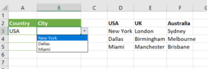
We can now copy from B3 to B4:B5 to complete the table.

If you are using SQL Spreads to manage data in SQL Server, there’s a great article here about using tables in SQL Server to populate drop-down lists in Excel: “Replace Key values with a Drop-Down list”.

Summary

XLOOKUP is a new Excel function that replaces VLOOKUP (and HLOOKUP).  Users experienced with VLOOKUP will be pleased to see that XLOOKUP addresses some limitations with VLOOKUP as well as adding some new features:

• XLOOKUP can look up data to the left of the lookup array (VLOOKUP can only look up to the right)
• XLOOKUP defaults to the more commonly used exact match option (VLOOKUP defaults to approximate match)
• XLOOKUP can work with vertical and horizontal data (HLOOKUP is no longer needed either)
• XLOOKUP can return multiple results
• XLOOKUP can perform a reverse search (last to first) (VLOOKUP can only perform first to last)
• XLOOKUP can return entire rows or columns (VLOOKUP can only return one value)

For users that have never used VLOOKUP, this article has introduced you to its new and improved replacement, XLOOKUP.  We’ve gone through several examples that show both simple and advanced uses of the function.  Even in its basic ‘exact match’ form, XLOOKUP is one of the most useful Excel functions and you’ll wonder how you managed without it before!

 

*This article was originally published on May 27, 2021 and was updated on March 2, 2022 to include additional information on the availability of XLOOKUP.